TROUBLESHOOTING LOW LEVEL VOLTGAGE
MEASUREMENT ERRORS
TROUBLESHOOTING >

Many articles evaluate different sources of error when measuring low voltage levels (e.g. ±10mV), yet seldom explain how to identify the cause of error, and if found, what to do about it. We will do this and show examples using a load cell sensor (pictured to the right) and an instruNet i423 digitizer.

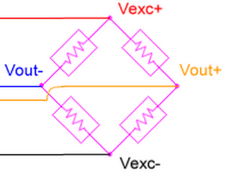
The instruNet digitizer is designed to attach directly to many different sensors including voltage, current, resistance, load cell, strain gage, thermocouple, and RTD. Our load cell sensor measures 0 to 2Kg of force and internally contains four 350 ohm resistors that are bonded to a metal plate that flexes when pressed, and in turn changes the resistor values. You can think of this as a sensor with a 350 ohm source impedance that receives a 3.3Vdc excitation voltage and produces a ±10mV signal with a 1.65Vdc offset. The data acquisition differential amplifier sees ±10mV and we will evaluate microvolt level errors. All pictures in this article are actual measurements from this setup. Below is a schematic of our sensor. Electrically, a load cell sensor is the same as a strain gage and mV/V pressure sensor.

We focus on the following sources of error:

• RFI Couples into Sensor Signal
• 50/60Hz Power Couples into Sensor Signal 
• Data Acquisition System Internal Noise
• Thermal Drift and Sensor Instability

SETUP
Normally sensors attach to a data acquisition system via a shielded cable; however, for the purposes of demonstrating RFI (radio waves coupling into signal wires), we break out the IN+ wire and induce an offending signal with a function generator. The function generator 5Vrms output is connected to a bare wire that wraps around the sensor IN+ wire 10 times. We place 270 ohms in series with the function generator output to facilitate 18mA through the offending coil (5Vrms / 270 = 18 mArms).

We also attach a dummy sensor to a 2nd measurement channel that is electrically similar to the load cell. It consists of four independent thin film resistors floating in air at the end of a cable, where the function generator is attached in the same way as the load cell. RFI couples more with increased source impedance; therefore, our dummy sensor has the same 350 ohm source impedance as the load cell. The 2nd channel is used to identify slight instability from within the load cell itself.

A 3rd channel is grounded with a 2cm wire between data acquisition IN+ and IN-, and between GND and IN+. This 3rd channel is used to determine the internal system noise and thermal drift of the data acquisition system itself. All experiments are conducted with an instruNet i423 card on its ±10mV measurement range using instruNet World Oscilloscope/Strip chart software. This card provides software selectable 6Hz and 4000Hz 2pole analog low pass filters, software selectable digital filters, and software selectable integration (averaging).

Many load cell manufacturers recommend an excitation voltage of 10V which pumps 285mW into the load cell (10^2/350 = 0.285). This creates heat and temperature drift; therefore we prefer to run at a lower 3.3V, which corresponds to a gentler 31mW.

RFI COUPLES INTO SENSOR SIGNAL

What is RFI?
RFI (radio frequency interference) involves radio waves that travel through air and couple into wires. This is explained by Maxwell’s equations that state that a change in wire #1 current (e.g. 60hz power wires) creates a magnetic field which flows through a loop of wire #2 (e.g. wires to sensor) and induces a current in that wire, which then converts to a voltage after traveling through resistance (referred to as "inductive coupling"). The effect of RFI increases with increased source impedance (source is less strong to fight RFI); therefore, high source impedances and low level measurements are the most challenging.

On/Off Switching RFI
When an offending signal in the vicinity of a sensor wire makes a low-to-high transition, an upward spike couples into the wire, and when it makes a high-to-low transition, a downward spike couples (or visa-versa if RFI flux is in opposite direction). This is why we sometimes see spikes on a digitized waveform -- they relate to an offending digital signal or device turning on or off.

Sinewave RFI
Alternatively, a sinewave can travel through air and couple another sinewave of the same frequency onto one’s signal. AM radio is approximately 1MHz and FM radio is approximately 100MHz, and both are notorious for entering the laboratory or factory.

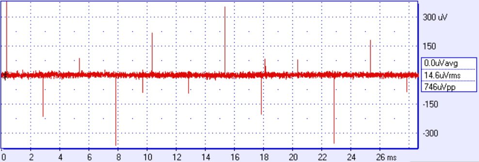
How to Detect RFI
Set up your data acquisition to digitize from one channel as fast as possible with all analog and digital low pass filters off and integration (averaging) off. Then view the resulting wave at different horizontal scales (e.g. 100μSec to 50mSec per full screen). Do this even if your ultimate experiment is to digitize multiple channels at a different sample rate with integration/filtering on. You might feel compelled to turn on filtering to make your signal look good. Yet for now, resist this temptation, and focus on learning more about your signal. The trick to understanding measurement error is to let go of your ultimate goal for a moment, and do some simple experiments. The below example shows 350μV spikes from a 200Hz square wave where we digitize 8k points at 166ks/sec from our 350 ohm load cell. instruNet is capable of very fast digitizing when only working with one channel and not switching channels.

How to Determine The Offending Source
While repeatedly digitizing oscilloscope traces, turn devices in the vicinity on and off (e.g. machine, pump, power supply), and view the effect on your digitized waveform. If you turn off a nearby power supply, and see spikes disappear, then that power supply is coupling into your sensor.

Through Air or Metal?
Is the offending signal traveling through air and coupling into your sensor cable, or does it travel through your ground wire? Try moving your sensor cable and look at the effect on the digitized wave. Does the position of the cable effect the plot? If so, RFI in the air is passing through a loop of wire (your cable) with a different physical geometry (different flux), and therefore changes. Change due to moving cable is the telltale sign of through-the-air RFI. Added cable shielding might help, in addition to several other techniques discussed below.

Are Ground Loops Making you Crazy?
Is your cable/sensor ground attached to external metal (e.g. device under test)? If so, physically disconnect and look at the effect on your signal. If your signal changes, then you know current is flowing along your ground wire due to an AC signal between your data acquisition ground and device under test ground. This is called a “ground loop” and is often fixed by electrically isolating the sensor (e.g. with i601). The AC voltage difference between grounds is often caused by changing power, which involves changing current on the ground return path and its associated voltage drop on that ground wire. A typical difference between grounds is 15mVac on top of 50mVdc. To measure this with a sensitive data acquisition system, attach IN+ to ground #1, attach IN- to ground #2, digitize one channel as fast as possible and view 100μSec to 25mSec per full screen.

Will Differential Amplifier Common Mode Rejection Save Me?
Data acquisition systems have differential inputs that measure the voltage difference between two inputs. All differential amplifiers have a specification for how much common signal on both inputs is rejected. A typical specification is 80dB rejection at 60Hz. This means that 1/10000th of 60Hz on both pins is seen as a differential signal. For example, connect IN+ to IN- with a bare wire, apply 60Hz 1Vrms between IN+ and GND, digitize, and you will see 60Hz 100μVrms between IN+ and IN-. The dirty little secret of data acquisition is this rejection gets worse by 20dB per decade, which means you get 1/1000 rejection at 600Hz, 1/100th at 6 KHz, 1/10th at 60 KHz and nothing beyond. Digital switching (e.g. spikes) often involve frequencies in excess of 60 KHz. Therefore, in many cases, amplifier common mode rejection will not save you, especially with digital switching RFI.

Will an Analog Low Pass Filter Save Me?
The below picture shows the effect of a 4KHz-2pole analog filter, which caused our 350μV spikes to decrease in amplitude to 15μV. We increased the plotted vertical resolution from 150μV/div to 12μV/div to better see the smaller spikes.

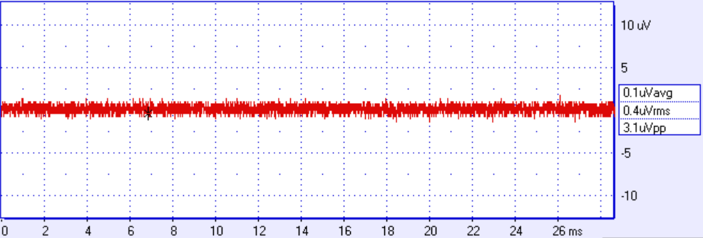
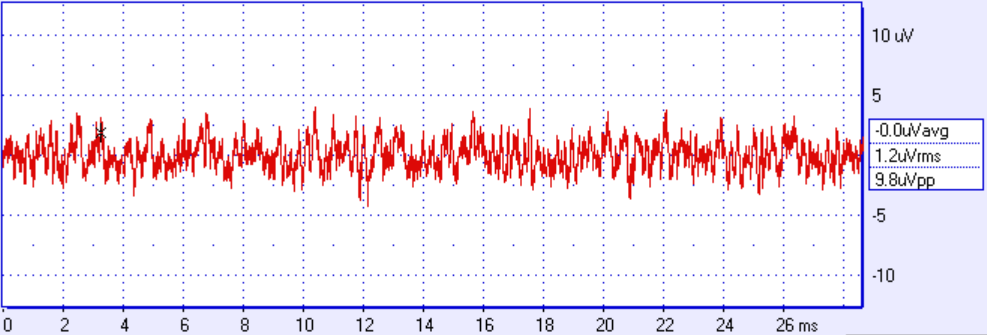
The below picture shows the effect of a 6Hz-2pole analog filter, which completely eliminates the spikes. The resulting waveform is 0.4μVrms of noise, which is the internal system noise of the data acquisition system itself when limited to 6Hz of bandwidth.

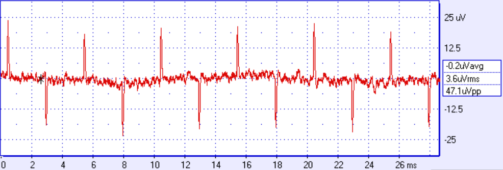
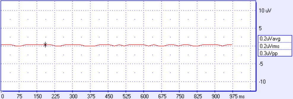
Will Software Integration Help?
Many data acquisition systems offer software integration (sometimes referred to as “averaging”) which involves reading the signal multiple times with an A/D converter and calculating an average for each point. For example, if one reads the signal every 6μSec for 16mSec then the measured value will be the result of averaging 2600 numbers. If your A/D converter produces 16-bit (±32K) integers and you sum 2600 of these to build an average, then your summation will be an integer between -82M and +82M, which is 27bits (2600*32K=82M). In other words, you increase the resolution of your 16bit A/D when you integrate. This does not necessarily mean your accuracy increases to 27bits due to multiple sources of error where each is typically in the 10bit to 18bit range. If you see an advertisement for a “24-bit” A/D converter, the same thing is occurring. Multiple digital values are summed to produces more numbers, yet not necessarily more accuracy.

The below picture shows the effect of integrating for 1mSec (160 A/D values averaged to make each point). Some of the 1msec integration bins include a spike from our 200 Hz square wave, and some don’t; therefore we still see some variation, yet at a reduced level.

Note that upward spikes cancel downward spikes when integrating, provided there is an equal number in each integration bin (i.e. N upward cancels N downward). The upward and downward do alternate since they relate to on/off switching. However, if you get N+1 upward and N downward in one integration bit, then you will get an offset from that last spike not having a partner to cancel with. If one spike is small relative to your other A/D points, the effect is negligible (e.g. if you average 2600 points and one of them is off by 100-fold, the effect of that one point is 100/2600 = 1/26th); however, if you have fewer good points or your bad point is large, then your integration is less effective.

The below picture shows the effect of integrating for 16.666mSec (2600 A/D values per point). This reduces our system noise to 0.2μVrms. Integrating for one power-line cycle (i.e. 1/60th of second = 0.016666 seconds) significantly reduces power-line noise due to the positive part of the power-line sinewave being canceled out by the negative part.

Software integration often reduces the maximum sample rate because the A/D needs to focus on reading one channel multiple times to get one point. In the above illustration for example, we integrate for 16mSec yet we also reduce the maximum sample rate from 166Ks/sec aggregate (all channels) to 60s/sec.

What to do if the sensor frequency is similar to the noise frequency?
If too much filtering rejects the signal of interest; consider better shielding, electrically isolating the sensor from the device under test, shorter sensor cable, and/or identify source of noise and reduce it.

50/60Hz Power Couples into Sensor Signal
A typical problem with low level measurements is the coupling of 60Hz (or 50Hz) power into the sensor signal.

How to Detect 50/60Hz Power Coupling
Digitize one channel as fast as possible with analog filters off, digital filters off, integration off; and look for a sine wave that is 16msec long (or 20ms with 50Hz power) while plotting 20mSec to 50mSec per full screen. Below is an example where we digitize 5k points at 166ks/sec. Notice the slight 60Hz sinewave. If our cable was longer, this would be larger.

Fixing The Power Problem
The below picture shows the effect of a 6Hz-2pole analog filter. This reduces 60Hz noise by a factor of 100. Two poles reject frequencies beyond the cut-off frequency by 40dB (100-fold) per decade (60Hz/6Hz = 1 decade). We end up with 0.4μVrms of system noise below 6Hz, which is mostly from the A/D converter.

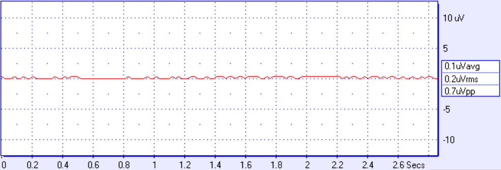
Alternatively, we turn off analog filters and instead integrate for 16.666mSec to reduce system noise to 0.2μVrms, as shown below.

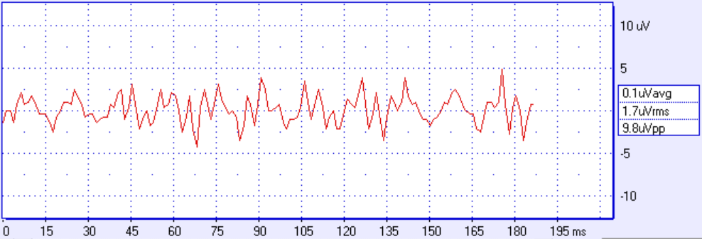
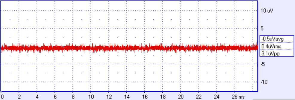
If your sensor signals are fast (i.e. > 60Hz) and you don’t want to filter out your signal of interest, then consider a digital band stop filter, shown below. We still see 1.2μVrms of data acquisition system internal system noise, yet the 60Hz sine is gone.

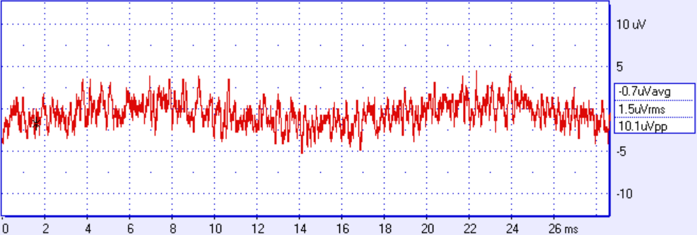
Data Acquisition Internal System Noise
All data acquisition systems have internal noise that is added to the digitized signal. This is due to a property of amplifiers -- they all add a little noise to their received signal. To see this, ground the input (wire from IN+ to IN-, and wire from IN+ to measurement system GND), digitize one channel as fast as possible with filter/integration off, and view 100μSec to 25mSec per full screen. The previous picture is an example of what you might see.

What To Do?

• This noise decreases with decreased bandwidth. For example, we measure i423 system noise on the ±10mV measurement range at 6μVrms with 125 KHz full bandwidth, 1.2μVrms with 4 KHz bandwidth and 0.4μVrms with 6 Hz bandwidth. So turning on analog filters can help.
• When you integrate (average multiple A/D values), noise decreases with the square root of the number of values that you average. For example, we measure i423 digitizer noise at 6μVrms with no integration and 0.2μVrms with 16mSec integration (2600 A/D values). In this example, we see a 30-fold reduction in noise (6 /0.2 = 30), which is similar to SQRT(2600) = 51.

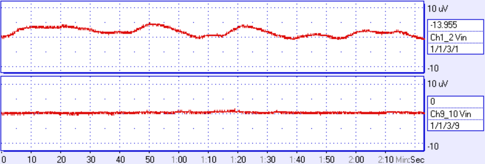
Thermal Drift and Sensor Instability
If your sensor is supposedly not changing and you see it change slightly over several minutes or several hours, then the question becomes, “what is the cause and how do we measure it?” The cause is typically due to one or more of the following: data acquisition system thermal drift, sensor thermal drift, or sensor instability.

Data acquisition systems drift slightly when their internal temperature changes. To see this, ground an input, digitize over 10 minutes, average each point for one power-line cycle to reduce noise (so we can focus on long term drift and not noise), gently heat the measurement system with a heat gun and view the digitized waveform with a small vertical scale (e.g. 2μV/div). After it warms, one can often command the system to recalibrate, and see the measurement move back to what one would expect.

Sensor thermal drift is similar. One can gently heat the sensor with a heat gun and watch it change.

Sensor instability is when a sensor changes yet not due to temperature and not due to a change in stimulus. The cause depends on the sensor itself. For example, a load cell might slightly relax mechanically over time after being stressed, and still stay within specification.

How To Measure Sensor Thermal Drift and Instability
Digitize two channels at a slow sample rate where you view 10 minutes per screen and integrate each point for one power-line period to reduce noise and focus on long term drift. One channel is connected to your sensor, and the other is connected to a resistor at the end of a cable, where the cable is similar to your sensor’s cable and the resistor is similar to the source impedance of your sensor (350 ohms in our case). Below is an example with our test setup. Notice our dummy sensor is stable, yet the load cell moves 5μV with no stimulus. It is not clear why it does this -- this low level change is not specified or described by the manufacturer of the sensor. This 5μV is still within the specified accuracy of the sensor. If this is a problem, consider a more accurate sensor.

To better characterize long term changes, one can simultaneously digitize a sensor and dummy resistor with one power-line cycle integration for several minutes to several hours with:

• No stimulus
• Turn on air conditioner or room heater
• Apply heat with heat gun to sensor and then to data acquisition system
• Turn on external devices (e.g. power supply, machine, pump)

Conclusion
One can often characterize sources of low voltage errors by conducting a variety of experiments with analog filters, digital filters, and integration while digitizing from the actual sensor, a dummy cable/resistor, and a grounded input.